Introduction

The salinity of the Sound is largely determined by the discharge of the Connecticut (O’Donnell et al., 2014). The salinity is extremely important to the Sound ecosystem because the distribution is not uniform and the density gradients that arise drive both very significant horizontal circulation and contribute to the inhibition of vertical mixing. The Hudson River also has an effect, however, since the salinity at the western end of the East River is determined by the flow rate in the Hudson. The net freshwater flux is thought to be small, in an annual average sense, relative to the Connecticut River, but at the western end of the Sound where seasonal hypoxia is common (see O’Donnell et al., 2014), it has an important influence on both the vertical stratification and the non-tidal current structure. The archive of direct salinity measurements in the Sound is very limited; however, long records of flow rate have been acquired and understanding their trends is likely to provide insight into their impact on the ecosystems.

Gay et al. (2004) showed that Connecticut River is the dominant source of fresh water to LIS, contributing 75% of the total gauged discharge. In winter, precipitation in the form of snow collects in the hills and mountains of the New England states. Much of this area is in the watershed of the Connecticut River. As a result, the Connecticut River usually experiences its smallest river flows in January-March. As temperatures rise in the spring, precipitation turns to rain and the snow and ice melts. This leads to higher runoff. The periods of high flow is termed the spring freshet.

This figure shows the average seasonal cycle in the discharge measured at the U. S. Geological Survey’s gaging station at Thompsonville, CT (from O’Donnell et al., 2014). On average, the peak flow occurs in April. However, the variability in the time of the peak flow is substantial and this leads to the large standard deviations and a broad peak in the monthly average discharge that spans March-May. The average annual discharge is approximately 500 m3/s (shown by the horizontal line). Clearly, during nine months of the year the monthly mean flow is below the annual average.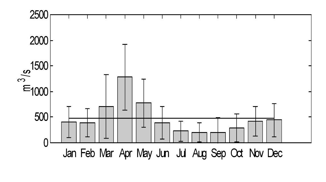

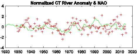
 There is substantial inter-annual variation in the discharge of the river that is driven by regional scale meteorological variability, and Whitney (2010) has shown that the Connecticut and several other rivers of the eastern United States correlate with the North Atlantic Oscillation (NAO) index (Hurrell, 1995). Using the same record, O'Donnell et al. (2010) showed that the day of the year by which 50% of the annual discharge has passed the gauge, the "center of volume flow," has become earlier at a rate of 9 ± 2 days/century. That the fresh water stored in the winter ice and snow pack arrives at the ocean through the Connecticut River earlier than in the past is consistent with the analysis of unregulated New England rivers and streams reported by Hodgkins et al. (2003) and is, therefore, likely to be a consequence of regional meteorological fluctuations rather than changes in watershed management.

Changes in the magnitude and timing of the freshet and the mean annual discharge will have significant implications for patterns of circulation and sedimentation in the Sound, and may also have implications for some aquatic and marsh species along the shore. Flooded fields and marshes during the freshet provide critical feeding habitat areas for migratory waterfowl and fish. The freshet also carries a large fraction of the annual sediment load to the Sound and the timing and magnitude may have long term impacts.

Summary

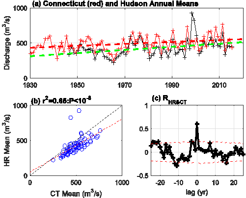
We examined the trends in the discharge in the Connecticut and Hudson Rivers. These both have a major influence on the salinity in LIS and consequently, the patterns of circulation and mixing. The effects are quite different since the location of the sources and the mechanism that control the distributions are quite different. Our analysis has demonstrated that the character of river discharge patterns is very similar in the Connecticut and Hudson and that they have exhibited large decadal-period oscillatiWe showed that the annual discharge in both rivers was increasing. on and secular trends during the last century. The decadal scale fluctuation in the two rivers were found to be significantly correlated at zero lag and negatively correlated at approximately 10 years, indicating that the forcing of the long period fluctuations affected the watersheds of the two rivers in a similar manner. However, despite the similarity in the character of the variations in the records, the correlation with the NAO index showed was not found to be significant. This seems likely to be a consequence of the highly variable lags in the relationship between precipitation and streamflow in very large basins.
We also conformed an earlier finding that the spring freshet was occurring earlier in the spring (the WSCV was decreasing) and was advancing at a rate of 8 days/century. The Hudson was shown to be undergoing a similar trend though at a slower rate.

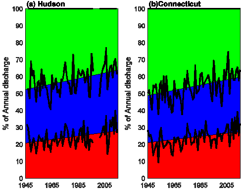
The most significant and novel result of the analysis is that the streamflow in the spring was stable and that the discharge in the low-flow months (June-December) was increasing. The rate of increase has led to almost a doubling of the amount of water reaching New York Harbor and LIS in these months. To more clearly illustrate the magnitude of the changes that have occurred we divided the year in to three phases based on the average seasonal cycle. The “low” phase extends from June to October when both the 5-day and monthly means are below the annual average. The “average” flow interval occurs in November to February and the “high” phase is March to May, when the spring freshet occurs. Note that these intervals are not of equal length. We then computed the total volume passing the gages in the three intervals each year and calculated the fraction of the annual freshwater volume occurring in each.

The lower black line shows the fraction of the annual flow occurring in the “low” phase. The boundary between the red and blue areas was obtained by linear regression of the low phase discharge fraction against time. Figure 4.10b shows the same property for the Connecticut River. The upper black line in Figure 4.10a and b shows the evolution of the sum of the discharge fraction during the below-average and average phases, and the boundary between the blue and green areas is the temporal trend in the sum of the fractions. The distance from the upper black line to the top of the graph represents the spring discharge contribution to the annual cycle. The green, blue and red areas then each represent the contribution of the three phases (high, average and low) of the discharge cycle to the delivery of fresh water to the estuaries.

 In 1945, approximately 50% of the freshwater arrived in the estuary during the three months of the high phase. As a fraction of the annual flow, it has diminished by almost 15% in the Hudson and 10% in the Connecticut. Both the other phases have expanded their contributions. It is unclear why this has happened. Since patterns are the same in both watersheds, it seems unlikely that there has been a reduction in the diversion and changes in precipitation are more likely. The implications of these changes are unclear and the issue will require further study. The availability of more freshwater in the Hudson in the summer may, for example, decrease the salinity and increase the stratification in the western Sound.

References

Bradbury, J.A., S.L. Dingman and B.D. Keim. (2002). New England Drought and Relations with Large-Scale Atmospheric Circulation Patterns. Amer. Water. Res. Assc. V 38, No. 5, 1287-1299

Hodgkins G.A., R.W. Dudley and T.G. Huntington (2003). Changes in the timing of high river flows in New England over the 20th Century. J. Hydrology V278, 244–252

Gay, P.S., J. O’Donnell and C.A. Edwards (2004). Exchange Between Long Island Sound and Adjacent Waters J. Geophys. Res. 109, C06017, doi: 10. 1029/2004JC002319.

Hurrell, J.W. (1995). Decadal Trends in the North Atlantic Oscillation Regional Temperatures and Precipitation. Science 269: 676-679.

Hurrell, J.W. and C. Deser (2009). North Atlantic climate variability: The role of the North Atlantic Oscillation. J. Mar. Syst., 78, No. 1, 28-41 - See more at: https://climatedataguide. ucar. edu/climate-data/hurrell-north-atlantic-oscillation-nao-index-pc-based#sthash. 77h8RnZx. dpuf

O'Donnell J, J. Morrison and J. Mullaney (2010). The expansion of the Long Island Sound Integrated Coastal Observing System (LISICOS) to the Connecticut River in support of understanding the consequences of climate change. Final Report to the CTDEP, LIS License Plate Fund, 20pp.

O'Donnell, J., R.E. Wilson, K. Lwiza, M. Whitney, W.F. Bohlen, D. Codiga, T. Fake, D. Fribance, M. Bowman, and J. Varekamp (2014). The Physical Oceanography of Long Island Sound. In Long Island Sound: Prospects for the Urban Sea. Latimer, J. S., Tedesco, M., Swanson, R. L., Yarish, C., Stacey, P., Garza, C. (Eds.), ISBN-13: 978-1461461258

Whitney, M.M. (2010). A study on river discharge and salinity variability in the Middle Atlantic Bight and Long Island Sound. Cont. Shelf Res 30:305-318

Willmott, C.J., S.G. Ackleson, R.E. Davis, J.J. Feddema, K.M. Klink, D.R. Legates, J. O'Donnell, and C.M. Rowe (1985). Statistics for the Evaluation and Comparison of Models. J. Geophys. Res. 90: 8995-9005.

Back to top