Introduction

The air temperature has a direct effect on many coastal ecosystems. The flora and fauna of marshes and the rates of geochemical processes are all directly influenced. It is well established that the global average temperature has been increasing and is projected to increase more rapidly in the future (Kirtman et al., 2013). However, the mean temperature is not always the most important statistic of the environment in many ecological systems. For example, the time of the year that the temperature is above a threshold is important to insects and their predators, and many species of plants. We showed in Chapter 1 that the summer mean temperature at Bridgeport, Connecticut, has increased at a rate of 0.8 ^oC/century; however, we uncovered a much earlier evaluation. The first assessment of the climate change in Connecticut was published in by Loomis and Newton (1866). They carefully examined the temperature measurements that had been recorded by a variety presidents and professors of Yale College in New Haven between 1779 and1865, and developed corrections to account for the time of day of the measurement. They then considered whether the annual, seasonal and monthly mean temperature had changed between the intervals 1779 to 1820, and 1820 to 1865. They also reported an analysis of the variation in the date of the last frost of spring and the first frost of fall. Since the records of direct observations of frost were unreliable, they used the occurrence of temperatures lower that 40 ^oF (or 4.4 ^oC) as more convenient metric. They showed that this proxy was a reasonable predictor of frost when observations were available.

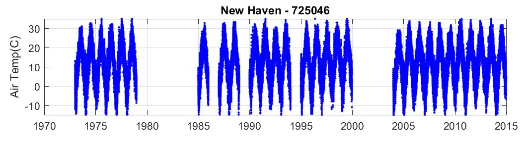
Since we have now have access to the hourly observations of air temperature in New Haven, a comparison of 30 years of recent observations to those completed over 150 years ago is appropriate.

Summary and Discussion

We have presented an analysis of the air temperature fluctuations in a coastal area close to Long Island Sound. The data was extracted from a NOAA data base and then examined for inconsistencies. These were eliminated where possible.
We then transcribed old observations from an obscure source that dated back to 1779. These data had been assiduously reviewed by the collators considering the era in which they worked. Comparison of the mean monthly temperature has revealed that there has been a warming of between 2 oC and 4 oC in the last 200 years. The larger values apply to the winter months (November-February) and the smaller values to April-August. The larger values are statistically significant.
	a) shows the annual cycle of air temperature at New Haven, CT. The solid black line shows the monthly mean computed from the data from Tweed-New Haven Airport and the dashed lines above and below it show the standard error of the means. The green and red lines show the estimates from the analysis of Loomis and Newton (1866). They are almost identical. In (b) the difference between the black and the average of the green and red lines is represented by the ‘+’ symbols. The red line shows value the difference would have to exceed to be different from 0 at the 95% confidence level assuming the all the estimates of the mean are independent. The green line shows the level if substantial autocorrelation is assumed.
We also examined the data for evidence of trends in the day of the year that frosts end in the spring, and start again in the fall. Loomis and Newton (1866) had published the mean for the period 1779-1865. We find that the frosts end earlier and begin again later by 16.1 and 19.7 days, effectively lengthening the warmer season by almost 36 days.
	The day of the year when the last temperature value below 4.4 oC (40oF) was observed in the data from Tweed-New Haven airport is shown in by the red ‘+’ symbols. The first day in the fall when the temperature falls below 4.4 oC is shown by the blue circles. This threshold was chosen to represent condition suitable for frost. The red and blue lines show the mean date of these thresholds were crossed in the data records from 1779-1820 (red and blue solid lines) and 1820-8165 (red and blue dashed lines).

 There have been global (Kirtman et al., 2013) and regional (Horton et al., 2014) analyses that have detected significant changes in air temperature. However, it is very difficult to detect changes at a single location. The availability of three decades of high quality air temperature data at Tweed-New Haven Airport, and the legacy of careful measurement several times a day by the scholars at Yale in the 18^th and 19^th century, allows this analysis. That the results are broadly consistent with those of the regional and global analyses add confidence that the missing metadata is not an overwhelming problem.

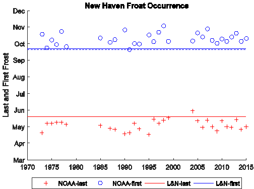
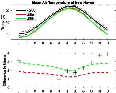
One consequence of this warming is the substantial decrease in the fraction of the year that frost is likely. At the end of the 17^th century the frost-free duration was 125 days. Now it is 161 days, an increase of 29%. Gaps between other temperature thresholds have experienced similar increases. Examination of the seasonal temperature cycle in Figure 3.2a shows that the transitions form February to June and September to December are almost linear. The effects of warming on the length of an interval above any temperature between 5 and 20 ^oC can be easily estimated.

It is also interesting and significant to note that warming appears to be larger in the winter. This is likely due to the radiative equilibrium that occurs in the summer when the loss of heat at night is large. Monitoring in the winter is more likely therefore to yield a detectable effect earlier.

The ecological consequence of the lengthening of the summer have not been very extensively investigated. It appears likely that plant and insects will benefit substantially. For short lived organisms, a few weeks or a month may be enough time to increase the number of generation cycles per year. The long period (decadal) variations in temperature that overlie the long term trend we focus on here may only a have an amplitude of a few degrees, but since we find that a 2-4 ^oC warming increases the duration between frosts by 29%, it appears likely that the effects of these decadal-scale variations can be similarly amplified. This effect deserves further attention from ecologists.

References

Horton, R., G. Yohe, W. Easterling, R. Kates, M. Ruth, E. Sussman, A. Whelchel, D. Wolfe, and F. Lipschultz (2014). Ch. 16: Northeast. Climate Change Impacts in the United States: The Third National Climate Assessment, J. M. Melillo, Terese (T.C.) Richmond, and G. W. Yohe, Eds., U.S. Global Change Research Program, 16-1-nn.

Kirtman, B., S.B. Power, J.A. Adedoyin, G.J. Boer, R. Bojariu, I. Camilloni, F.J. Doblas-Reyes, A.M. Fiore, M. Kimoto, G.A. Meehl, M. Prather, A. Sarr, C. Schär, R. Sutton, G.J. van Oldenborgh, G. Vecchi and H.J. Wang (2013) Near-term Climate Change: Projections and Predictability. In: Climate Change 2013: The Physical Science Basis. Contribution of Working Group I to the Fifth Assessment Report of the Intergovernmental Panel on Climate Change [Stocker, T.F., D. Qin, G.-K. Plattner, M. Tignor, S.K. Allen, J. Boschung, A. Nauels, Y. Xia, V. Bex and P.M. Midgley (eds.)]. Cambridge University Press, Cambridge, United Kingdom and New York, NY, USA.

Loomis, E. and H.A. Newton (1866) On the mean temperature and on the fluctuations of temperature at New Haven, Connecticut, 41^o 18’N, 72^o 55’W of Greenwich. Connecticut Academy of Arts and Sciences, Volume 1 Article 5 p 194-246.

Back to top